Working with what you have – a practical protocol for building a local heatwave threshold when the data are incomplete

Article 3 of the Heatwaves series | HansOnResilience.com Hans Guttman | July 2026

A country or region is increasingly experiencing heatwaves, which cause deaths, decline in productivity — in both labour and agriculture — and disruption to infrastructure and services. An early warning system is needed, or the one in operation needs to be enhanced. How do you go about doing this?

Two previous articles in this series explained why a universal temperature number does not serve you well, why a locally calibrated, anomaly-based heatwave threshold matters for impact-based forecasting, and which index is likely to give the most meaningful result — the Excess Heat Factor (EHF). The temperature component T-EHF, and its humidity-inclusive extension, the HI-EHF.

Article 1 “Heat kills more than almost any disaster — so why can’t we define it?” Click here

Article 2 “Defining heat where you live — a framework for localised heat indices” Click here

But where do you start? Thirty years of clean daily temperature records may not be available. There are records — a few good stations in major cities, some rural stations with gaps, a network that has been inconsistently maintained. What do you actually do? That is the question this article tries to answer.

The academic literature on heatwave indices is extensive and growing fast. This article does not add to that body of knowledge; instead, its aim is a step-by-step protocol for a practitioner working under real resource constraints in a data-limited environment — the case in many countries in the Global South where heatwave problems are acute and increasing. I hope meteorologists, public health officials, and disaster risk reduction practitioners who need to get something operational will find it useful.

Before you start, if you do not have the context yet, read the two earlier articles [links] in this series, particularly the argument for locally calibrated, anomaly-based thresholds over fixed absolute temperatures, and the EHF framework. The guidance here is based on access to – daily mean temperature derived from daily maximum (Tmax) and minimum (Tmin) observations. Measures of relative humidity are needed in the humid tropics or subtropics. Everything else builds on that. You also need a computer capable of basic data analysis and an internet connection. Beyond that, the approach is designed to work with very limited resources.

The data problem, stated plainly

The Excess Heat Factor (EHF), as originally developed by John Nairn and Robert Fawcett at the Australian Bureau of Meteorology, requires a baseline of 30 years or more of daily temperature records to calculate a stable threshold distinguishing a severe heatwave from a low-intensity one (Nairn and Fawcett, 2015; Nairn, Ostendorf and Bi, 2018). The 30-year requirement follows the World Meteorological Organization’s standard for climatological standard normals — the averaging period long enough to characterise a location’s typical climate with statistical stability.

In many countries across South and Southeast Asia, that record simply does not exist in usable form. Station networks were sparse or inconsistently maintained through much of the second half of the twentieth century. What records exist may be on paper (not digital), may have significant gaps, may cover only part of the country, or may reflect instruments and observation practices that changed over time without adequate documentation — facts on the ground rather than failures of intent.

The result is a practical bind: the rigorous approach requires data that many services do not have, and the alternative — a fixed absolute temperature threshold — produces a number with limited local meaning and no connection to the acclimatisation baseline (or how “used to” the population, service delivery and infrastructure is to ambient/normal temperatures) or cumulative heat stress that actually drive mortality, crop failures and other impacts. Is there a credible middle path?

There is, and it requires being precise about what ‘incomplete data’ actually means in different situations and choosing the appropriate response for each. Station data is always the primary input; ERA5 reanalysis (more on that later) is a fallback used to supplement or substitute for it, never a default starting point. The remainder of this article sets out that response as a practical protocol, structured as a decision tree running from node A to node L.

What WMO actually says about shorter records

An important clarification is worth making early, because it provides the “regulatory” grounding for what follows. The WMO does not say that 30 years of station records are required for all climate statistics. It says they are required for climatological standard normals — a specific, formal category. The WMO Technical Regulations define a separate, lower-tier category called “period averages”: averages of climatological data computed for any period of at least ten years, starting on 1 January of a year ending in the digit 1 (WMO, 2017). That ten-year floor is the WMO’s own regulatory minimum for climate statistics. It does not give the stability of a 30-year record, but it is not outside WMO-recognised territory, and it means there is a defensible, well-documented framework for working with shorter records — provided the limitations are explicitly acknowledged.

The practical protocol: a decision tree from data to threshold

A twelve-step path and a decision tree shown in Figure 1.

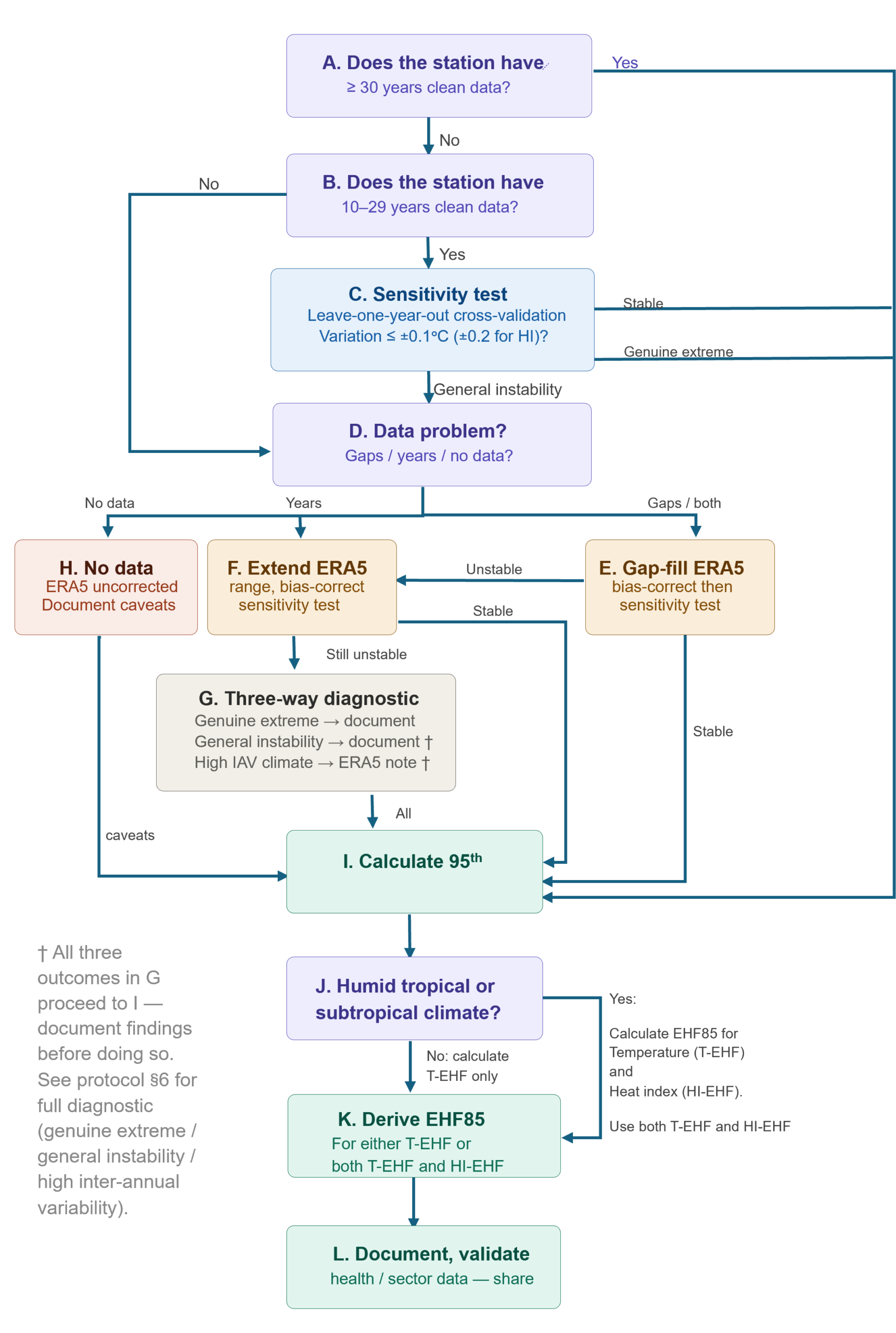
Figure 1: Decision tree for the protocol.

The decision tree serves two purposes: 1. it forces an explicit choice about which starting condition applies to your station network, and 2.it makes clear that every pathway — however constrained the starting data — converges on the same next step, deriving a locally valid 95th percentile threshold. What follows is a short description of each node. Calculation detail can be found in the annexes referenced at each node, so a reader who only needs the operational logic is not required to work through the equations to get it.

Node A — Do you have 30 years or more of clean daily Tmax/Tmin data?

A record of this length meets the WMO/Nairn and Fawcett “gold standard”. No sensitivity test is required, and no degree of internal variability in a record this long should divert you to the ERA5 pathway — a 30-year clean station record is treated as ground truth in this protocol. Go directly to node I. (“Clean” is defined in Annex A.)

Node B — Do you have 10–29 years of clean daily Tmax/Tmin data?

This is the WMO’s “period average category” — short of a full climatological normal, but a recognised statistical category in its own right (WMO, 2017). Proceed to node C.

Node C — Run the sensitivity test

Apply a leave-one-year-out cross-validation to the station record: remove each year in turn, recalculate the 95th percentile threshold, and compare it against the full-period value. The method, its tolerance bands, and a worked illustration are set out in Annex B. A stable result sends you to node I. Note that a record can also fail on internal consistency grounds even where the raw completeness percentage looks acceptable — see Annex A. An unstable result splits two ways: if the instability traces to a single, identifiable extreme year, document it and proceed to node I; if the threshold moves regardless of which year is dropped, the instability is general and you proceed to node D.

An unstable result splits two ways: if the instability traces to a single, identifiable extreme year, document it and proceed to node I; if the threshold moves regardless of which year is dropped, the instability is general and you proceed to node D.

Node D — Diagnose the primary data problem

Node D is a triage point, not a calculation. Establish what is actually “wrong” with the record (what causes the instability): gaps within an otherwise adequate span of years, an insufficient total number of years, or both. Gaps alone send you to node E. An insufficient span alone sends you to node F. If you have both gaps and a lack of years in the record, this sends you to E and then F in sequence. If you have no usable station data at all, you go to node H.

Node E — Gap-fill using ERA5, then re-test

Fill the missing gaps/periods in the station record with bias-corrected ERA5 values for the corresponding grid cell (method in Annex C), then re-run the sensitivity test described at node C. A stable result sends you to node I. If instability remains, proceed to node F.

Node F — Extend the record using bias-corrected ERA5, then re-test

Where the station record is simply too short, extend it — backwards in time, or by adding parallel years — using bias-corrected ERA5 data, following the same correction procedure (Annex C). Re-run the sensitivity test. A stable result sends you to node I. If instability persists even with an extended, bias-corrected record, proceed to node G.

Node G — Run the three-way diagnostic

Node G exists for the case where neither gap-filling nor range extension has produced a stable threshold. Rather than treating this as a dead end, the protocol asks you to establish why the record is unstable, because the appropriate caveat differs across three distinct causes: a genuine extreme event distorting the record; general statistical noise; or a climate that is legitimately highly variable year to year (Mongolia’s continental interior is a useful illustration — even long records there show greater inter-annual swings in summer temperature than a maritime tropical setting does). The diagnostic procedure is set out in Annex D. Whichever of the three applies, document it and proceed to node I with the relevant caveat attached.

Node H — No usable station data — use ERA5 uncorrected

Where there is no local station data to validate or correct against, use ERA5 directly, documenting the known regional biases for your area (Annex C) as an explicit caveat. Proceed to node I.

Node I — Calculate the 95th percentile threshold — the convergence point

Every pathway — station data alone, gap-filled, range-extended, diagnostically caveated, or uncorrected ERA5 — arrives here at the same calculation: derive the 95th percentile of daily mean temperature for each calendar day, using a 15-day moving window pooled across the baseline years (method in Annex E). Proceed to node J.

Node J— Is the climate humid tropical/ subtropical?

If yes, run T-EHF and HI-EHF in parallel. Temperature-only EHF under-detects a substantial share of severe heat events in humid climates, and HI-EHF under-detects a comparable share of dry ones — in Darwin, Australia’s wet tropics, roughly 42–63% of severe humid heatwave events were missed by temperature alone, and 25–32% of severe dry events were missed by Heat Index alone (Nairn, Moise and Ostendorf, 2022).

If no, use temperature-only, the T-EHF is sufficient on its own. Either way, proceed to node K.

Either way, proceed to node K.

Node K — Derive the severity threshold – the EHF85 (T-EHF85 and HI-EHF85 if needed)

Run the full EHF calculation (for T-EHF and for HI- EHF as appropriate) across the baseline period and take the 85th percentile of all positive EHF values, see Annex F. This is your local severity threshold, distinguishing low-intensity from severe heatwave days — the statistical rationale for the 85th percentile is set out in Annex G. Proceed to node L.

Node L — Document, validate, and share

Produce a short technical note recording every methodological choice — which ERA5 product, which baseline period, which stations were used for correction, the sensitivity test result — then validate the threshold against whatever independent evidence exists and share the methodology with your WMO Regional Climate Centre and the Global Heat Health Information Network. BUT this is not only a health-sector exercise. Agricultural services often hold documented crop and livestock heat thresholds; power utility engineers can quantify the loss of evaporative cooling efficiency at high heat and humidity levels. Both can corroborate and/or refine the threshold you have derived. Details are in Annex I.

From threshold to warning: the operational chain

The threshold is not the end of the process; it is the beginning of the operational one. A number in a technical report does no protective work on its own. What converts it into lives saved, or crop failure avoided, is the chain from detection to action. Integrating the EHF calculation into a daily operational workflow — so that an automatic flag fires when the calculation is run on forecast as well as observed data — is the first link in that chain. Before that flag is built, it is important to note that a positive EHF or HI-EHF reading only means something within the relevant window of concern for the sector using it. For human health, that means the local hot season. A flag firing on an anomalously mild winter week is a statistical artefact of the day-specific method, not a heatwave, and should not trigger the downstream actions described below. See Annex E for the underlying reasoning, and Article 2 for how windows of concern differ by sector.

The logic of that flag, and why it can give a two-to-five day warning window rather than a retrospective identification of events, is set out in Annex H. A separate piece is planned on how AI-based forecasting tools can help automate this step once the underlying threshold is in place; Annex H covers only the logic, and the calculations of the thresholds, not the automation.

That warning window needs to connect to pre-agreed action protocols: who receives the warning, what they do with it, and which agencies are responsible for which actions — cooling centres, checks on elderly residents, adjusted outdoor work schedules, hospital surge capacity, lowering electricity generation to not overheat generating stations, prepare for impacts of crop failure, prevent livestock stress and deaths. Those questions are the subject of a future article in this series and hopefully supported by the UN’s Extreme Heat Risk Governance Framework and Toolkit (mentioned in Article 1).

The point here is that the threshold and the protocol are not the same thing, but they cannot be designed in isolation from each other. How sensitive a threshold should be depends entirely on what “firing it” costs — and that cost is set by the protocol, not the statistics. A threshold that fires on every warm week is only a real problem because someone then has to act on it: opening cooling centres, redeploying health workers, or standing down outdoor work crews on what turns out to be a false alarm. The sensitivity that’s tolerable for a simple advisory is not the sensitivity that’s tolerable for a hospital surge-capacity call-out. Set the threshold too conservative instead, and it only fires once people, animals, crops or infrastructure are already in distress — which defeats the purpose of an early warning system in the first place. Deciding where between those two failure modes a threshold should sit is therefore not a purely statistical question; it depends on what the protocol actually asks people to do.

What this protocol cannot do

It is worth being direct about the limitations of this approach, because practitioners operating under resource constraints are often pressured to oversell what they have. The threshold derived through this protocol is a workable operational tool; it is not a validated emergency response product. A fully validated heat threshold — one you could confidently quote in a public health paper, for example — would be derived from a long, high-quality station record, bias-corrected against local conditions, and retrospectively validated against cause-specific mortality data linked to identified heatwave events. That level of validation requires data and specialist skills that most services in the region cannot currently provide. The approach here is the “best available alternative given what exists”, a practical approach.

Two uncertainties deserve explicit acknowledgement. First, the choice of baseline period matters: moving a shorter than “30 years to present” baseline by ten years can shift the apparent frequency of warm extremes by a meaningful margin, because the 1991–2020 baseline is warmer than the 1981–2010 one (Thomas et al., 2023). Whatever baseline is used, document it visibly, and be cautious about comparing heatwave frequency counts across studies using different baseline periods. Second, ERA5’s performance in very data-sparse regions — complex topography, small islands, interior regions with few assimilated observations — is less reliable than in well-instrumented areas. The validation step in Annex C should be taken seriously in those settings.

Neither limitation is a reason not to proceed! The limitations are the reasons to be honest about what you have and to plan for improving the evidence base over time. A ten-year ERA5-based threshold with a documented sensitivity test and a clear methodology note is vastly more useful — than no threshold at all (with all the caveats).

The technical minimum and the optimal: a summary

Component	Technical minimum	Optimal
Temperature data	ERA5 daily Tmax + Tmin (derived mean)	≥30 years quality-controlled station records + ERA5 for gap-filling
Humidity data	ERA5 dewpoint temperature (derived RH) for HI-EHF	Station RH records ≥30 years
Baseline period	10 years data, filled in with ERA5 as needed (WMO ‘period average’ floor), with sensitivity test	≥30 years, ERA5 bias-corrected against station records if needed
Bias correction	Documented ERA5 biases for the region; no correction if <5 years overlap	Quantile mapping (T-EHF); multivariate MBCn (HI-EHF), ≥5 years overlap
Index applied	T-EHF (dry-bulb temperature only)	T-EHF and HI-EHF in parallel; operational threshold on whichever gives the stronger signal
Statistical robustness	Leave-one-year-out sensitivity test on threshold (Annex B) on available records	For a full ≥30 years of quality-controlled station records, no other tests are needed
Impact validation (health)	Validate against existing independent evidence, e.g. partial mortality/hospital-admission records	Retrospective validation against mortality or hospital admission data covering past heat events
Documentation	Technical note with all methodology choices and ERA5 bias metrics	Peer review by WMO Regional Climate Centre or academic partner; published methodology

What still needs to happen at the international level

This protocol fills a gap. It does not resolve the gap. The underlying reason a “workaround” is needed is that NMHSs in many lower-income countries have been operating for decades without the resources to build and maintain the station networks that would make a full 30-year, high-quality baseline achievable. That is a governance and investment failure, not a technical one, and it will only be addressed by sustained investment in observational infrastructure — the kind of investment UN’s Early Warning For All (EW4All) agenda is hopefully able to catalyse.

There is also a methodological gap at the international level that no amount of local improvisation can fully substitute for. The joint WMO/WHO 2015 guidance on heat-health warning systems (WMO-No. 1142) remains the operative technical document for NMHSs developing heatwave monitoring systems, and it is now over a decade old (WMO signalled an intention in 2023 to update this guidance through the EW4All initiative, but no successor document has yet been published. Hopefully I am proved “wrong” in this context soon). It does not address the data substitution approaches described in this article — ERA5 as a long-record backbone, the HI-EHF extension for humid tropical environments, or the minimum viable baseline period recognised under WMO’s own technical regulations. The governance frameworks produced at COP30 in 2025 are a step forward on institutional coordination, but they do not provide operational methodology. Until updated operational guidance for NMHSs in data-limited tropical settings exists, each service must construct its own justification. The protocol here hopefully gives that justification a grounding in an adaptation of peer-reviewed practice.

Until that practical guidance exists, the best available substitute is transparency: if you use this protocol, document every step, acknowledge every limitation, and share your methodology widely. A community of NMHSs using comparable, well-documented approaches is more valuable than a set of formally endorsed but inaccessible thresholds — and it creates the evidence base that will eventually make the formal guidance possible.

Annex A — Defining “clean” data

For nodes A and B, a daily temperature or humidity record is treated as “clean” if it meets three conditions:

• Completeness: no more than a small proportion of days missing in any calendar year (a commonly used working benchmark is under 5%), and missing days are spread through the year rather than concentrated in one season — a station that is consistently offline every dry season for maintenance is not a clean record even if its annual completeness percentage looks acceptable.
• Documented continuity of instrumentation and observation practice: no undocumented station relocations, no undocumented changes in instrument type, observation time, or exposure (siting relative to buildings, vegetation, or paved surfaces) that could introduce an artificial step-change in the record.
• No unresolved discontinuities in the mean or variance of the series that cannot be attributed to a real climate signal — checked using standard homogeneity testing where feasible, or, at minimum, a visual review of the series for step-changes coinciding with known network events.

A record that fails any of these three tests is not disqualified outright, but it should not be treated as though it satisfies node A or node B directly. Route it instead through node D, where the specific problem (gaps, a genuine discontinuity requiring truncation, or both) can be diagnosed and handled explicitly.

Annex B — The sensitivity test: method, tolerance, and a worked illustration

Method: leave-one-year-out cross-validation. Remove each year from the baseline in turn, recalculate the 95th percentile threshold without it, and compare the result against the full-period value. Repeat for every year in the record.

Tolerance: the ±0.1°C (temperature) and ±0.2°C (Heat Index) bands used at nodes C, E and F are drawn from the one directly comparable published precedent — the Pearl River Delta study’s 10-year leave-one-year-out test (Zuo et al., 2026) — and should be treated as a practical starting benchmark rather than a universal statistical law. A location with a genuinely more variable climate may reasonably need a wider band, provided the reasoning is documented before the test is run; a location with a very stable maritime climate may reasonably use a tighter one. What matters operationally is that the tolerance is fixed and justified in advance, not adjusted afterwards to produce a “preferred” result.

A worked illustration: consider a 20-year station record where the leave-one-year-out test shows the threshold moving outside tolerance only when Year 19 is excluded — every other combination of 19 remaining years produces a stable result. That pattern points toward a single anomalous year rather than general instability. The next step is to check whether Year 19 corresponds to an independently documented extreme event — a recognised historic heatwave, a verified instrument fault, or similar corroborating record. If it does, node C’s ‘single confirmed genuine extreme’ branch applies: document the year and the reason, and proceed to node I with that note attached. If no such corroborating explanation exists — the year is simply measured unusually hot, with nothing independently confirming why — the safer classification is general instability, since an undocumented anomaly cannot be dismissed as an isolated event on the strength of the sensitivity test alone. That routes to node D.

Annex C — ERA5: access, validation, and bias correction

What is ERA5? ERA5 is the fifth-generation global climate reanalysis produced by the European Centre for Medium-Range Weather Forecasts (ECMWF) under the EU’s Copernicus programme, freely available at no cost. It provides hourly global data from January 1940 to the present at roughly 0.25° resolution (about 28 km wide path), from which daily Tmax, Tmin and relative humidity (RH) can be derived. ERA5-Land offers a finer, roughly 0.1° resolution (about 11 km wide path) and is particularly useful in areas of significant topographic variation.

Access. The Copernicus Climate Data Store (cds.climate.copernicus.eu) is the main access point; registration is free. Download 2-metre temperature (T2m) and 2-metre dewpoint temperature (Td2m), from 1981 to present as a minimum, or back to 1950 for a longer baseline.

Daily Mean Temperature (DMT) for EHF purposes is DMT = (Tmax + Tmin) / 2.

Relative humidity (RH) is not archived directly in ERA5 and must be calculated from the two downloaded fields, using the Magnus/Tetens approximation to derive RH from T2m and Td2m at each hourly timestep. Available at https://doi.org/10.1175/BAMS-86-2-225  (Accessed: July 2026). Daily RHmax and RHmin are then taken from the resulting hourly RH series, before averaging to Daily Mean RH (DMRH) for EHF purposes = (RHmax + RHmin) / 2.

Validating ERA5 against station data. This is a distributional comparison, not a leave-one-year-out test — the leave-one-year-out method (Annex B) checks the stability of a derived threshold; validating ERA5 checks whether the reanalysis is fit to build that threshold from in the first place. For each station with usable records, extract the nearest ERA5 grid cell and compare, over the overlapping period: the mean daily temperature (should be within roughly 1–2°C for most lowland tropical settings; a larger systematic bias should be documented and corrected); the variability of day-to-day temperature (ERA5 can under-represent this in very humid tropical settings, affecting percentile accuracy); and, most importantly, the 90th and 95th percentile of daily mean temperature. Checking both points, rather than the 95th alone, reveals whether any bias is roughly stable across the upper tail or widens toward the extreme — the latter is the more dangerous case, since the EHF threshold is built on the 95th percentile specifically, and a bias that grows with intensity will distort the threshold more than a flat, uniform offset would. A consistent gap of more than 1°C at the 95th percentile means bias correction is needed before ERA5 is used for threshold derivation. For relative humidity, ERA5 tends to show a dry bias in humid tropical coastal settings of around 4 percentage points (Zuo et al., 2026); this should be corrected jointly with temperature, not independently.

Bias correction. Where five or more years of station overlap exist, quantile mapping (statistical bias-correction to adjust values of simulated meteorological data so their statistical distribution matches observed historical records), is the standard method for temperature alone: compare the cumulative distribution of ERA5 values against the station record for each calendar month, and apply a correction factor that maps one onto the other. For HI-EHF, temperature and relative humidity must be corrected jointly, because Heat Index is a nonlinear function of both and correcting each independently can distort their relationship; the Multivariate Bias Correction (MBCn) method is the appropriate approach – available at https://doi.org/10.1007/s00382-017-3580-6  (Accessed: July 2026). It is the method used in the Pearl River Delta study (Zuo et al., 2026). Where fewer than five years of overlap exist, use ERA5 without local correction, documenting known regional biases explicitly (typically +0.5 to +1.5°C for mean temperature in humid tropical lowlands) and treating the resulting threshold as carrying greater uncertainty.

A note on humidity. Long, high-quality historical humidity station records are less commonly available in practice and gaps are more common. Humidity forecast skill is weaker than temperature forecast skill at the lead times useful for early warning. Two practical implications follow: where station humidity records are short or of uncertain quality, bias-corrected ERA5-derived relative humidity is likely your best available input for HI-EHF; and T-EHF should be maintained alongside HI-EHF even where the latter is operational, for continuity, for extended-range forecasting, and because the two indices catch different event types (node K).

Annex D — The three-way diagnostic (node G)

Node G applies only where a gap-filled or range-extended, bias-corrected ERA5 series still fails the sensitivity test. The purpose is to establish which of three distinct causes is at work, because each carries a different caveat:

• Genuine extreme variation: one or more years in the record contain a documented, independently corroborated extreme event (a recognised historic heatwave, verified against news or agency records). Document the event and its influence on the threshold, and proceed to node I with that caveat attached.
• General instability: no single year explains the result; the threshold shifts by a comparable amount regardless of which year is removed. This points to a baseline that is still too short or too noisy relative to the local climate’s natural variability. Document the uncertainty range explicitly and proceed to node I with that caveat.
• High inter-annual variability climate: the region’s climate is legitimately more variable year to year than the tolerance bands in Annex B assume — continental interior climates such as Mongolia’s are a useful reference case, where summer temperature swings between years are naturally larger than in a maritime tropical setting. Where this applies, note the wider ERA5 accuracy caveats that typically accompany such climates, document the variability explicitly, and proceed to node I with both caveats attached.

In practice, distinguishing between the three draws on the same evidence: independent event records (for the first), the pattern of the leave-one-year-out results across all years rather than just one (for the second), and reference to published regional climate variability studies or your Regional Climate Centre’s own characterisation of the area (for the third). Where more than one explanation plausibly applies, document all that are relevant rather than forcing a single diagnosis.

Annex E — Deriving the day-specific threshold (the 15-day moving window)

The 15-day moving window

A single calendar day, on its own, does not give you enough data to calculate a stable percentile. Thirty years of station records means only thirty values for ’15 July’ specifically — too small a sample for a reliable 95th percentile. The 15-day moving window solves this by pooling nearby days together.

The method: for each calendar day, take every daily value falling within a window centred on that date — typically 7 days before and 7 days after, so 15 days in total — across every year in the baseline. For 15 July, this means pooling all daily values from 8 to 22 July, for every year of the baseline period. With a 30-year baseline, that gives roughly 30 × 15 = 450 data points, enough for a statistically stable percentile estimate. Calculate the 95th percentile of that pooled sample: this is the day-specific threshold for 15 July.

Repeat this for every calendar day of the year (all 365, or 366 in leap years), each with its own centred 15-day window. The result is a smooth, slowly varying threshold curve across the year, rather than 365 independent and noisy single-day estimates. Critically, the window is centred on the calendar date, not drawn from the whole year — this preserves the seasonal cycle, so the threshold for a July day in the northern hemisphere summer stays distinct from a January day in winter, rather than being flattened into a single annual figure.

Edge cases at the start or end of the calendar year (e.g., a window centred on 28 December) wrap around into the following or preceding year’s data — this is standard practice and does not require special handling beyond ensuring your calculation script accounts for the wrap. This method is not specific to temperature. It applies equally to any suitably constructed daily variable — including a daily Heat Index (HI) value, where humidity is part of the local threshold. What differs by variable is not the moving-window method itself, but how you arrive at the single daily figure you feed into it. For temperature, that figure is DMT, the average of Tmax and Tmin. For Heat Index, constructing that daily figure is less straightforward, and depends on what data is actually available. The rest of this annex addresses that construction step specifically.

Day-specific thresholds and the window of concern

This protocol uses a day-specific threshold to calculate the T95— 365 separate values, one per calendar day, pooled via a 15-day moving window (the ETCCDI convention for percentile-based climate extreme indices; Zhang et al., 2005) — rather than a single annual value. This aims to make the threshold usable beyond human health. Because every calendar day has its own local baseline, each sector can define its own window of concern: the period of the year when an anomaly against that baseline actually translates into harm.

For human health, the window of concern is summer/hot season, which overlaps with the year’s absolute hottest temperatures. For agriculture, the window of concern may track the crop’s growth stage instead. Rice and other staples are most vulnerable during flowering, when a daytime temperature of roughly 33–35°C, or even a single night at 30°C or above, can cause spikelet sterility and crop failure — yet the same crop, outside flowering, tolerates 40°C or more without comparable damage. Under double- or triple-cropping systems, flowering can recur several times a year, and only the occurrences landing in an already-warm part of the calendar carry real risk.

This is a modification of Nairn and Fawcett’s (2015) original EHF, which uses a single T95 value calculated from all days of the year at once. The single value works well for human health, since it is set by the year’s hottest days and so naturally coincides with human health’s window of concern — but it would not register an anomaly landing outside the year’s hottest period, such as almond blossom in spring or a rice-flowering window in a cooler month, which is exactly when those sectors need the signal most. A day-specific threshold, compared only to its own local norm, can register an anomaly — an unusually mild but still cold winter week can be EHF-positive without being remotely harmful. But a positive EHF does not trigger only when the relevant window of concern is defined and applied, not assumed.

The operational rule that follows: a positive EHF or HI-EHF reading is only meaningful within the relevant window of concern for the sector applying it. For human health, that window is the local hot season, however defined for the location in question — a positive reading outside it should not be treated as a heatwave day for human health purposes. Sector-specific windows of concern for agriculture, energy, and other applications are addressed in Article 2, “One signal, multiple sectors — the promise and its honest limits”; this protocol’s default output should not be applied to those sectors without first establishing the relevant window of concern separately.

Constructing the daily HI value: three data scenarios

Heat Index cannot be calculated from temperature and humidity readings taken at different times, or combined from separately-recorded daily summaries — it must be calculated from a temperature and a relative humidity value measured at the same moment. This constrains how a daily HI figure can honestly be built, and the right approach depends on what a given station actually has.

Scenario 1: Hourly or frequent sub-daily data available

Where a station (or its automated weather station equipment) records temperature and relative humidity at least hourly, calculate HI at every reading. Identify the hour with the highest resulting HI value (HImax, typically the afternoon) and the hour with the lowest (HImin, typically just before dawn). Construct the daily HI figure as the average of HImax and HImin — directly analogous to how DMT is built from Tmax and Tmin.

This construction is deliberate, not a simplification of convenience. EHF’s design logic depends on capturing daytime peak stress and nighttime recovery failure as two distinct, equally weighted signals; a full 24-hour average of all hourly HI readings would blend these together and could produce an identical daily figure for a genuinely dangerous day (sharp afternoon peak, hot still night) and a much milder one (moderate, flat conditions all day). The HImax/HImin structure preserves the distinction that actually matters for the calculation. This is a reasoned design choice for this protocol, not an established consensus method — the Pearl River Delta study that pioneered HI-EHF at scale used a full hourly average instead, and no direct comparison between the two approaches has yet been published. Services adopting HImax/HImin should note this openly.

The overnight minimum deserves particular attention in humid climates. Relative humidity tends to rise as temperature falls overnight, so a night that appears to offer thermal relief by dry-bulb temperature alone may still leave little real physiological recovery once humidity is accounted for. HImin captures this more directly than Tmin alone, and is the main reason humidity matters as much on the recovery side of the calculation as on the peak-stress side.

Scenario 2: Only one daily humidity reading, but ERA5 (or equivalent reanalysis) available

Many stations recording only one relative humidity reading per day take it at a standard daytime observation hour. Pair that reading with the temperature recorded at the same time to construct an “honest” HImax figure for that day. The harder problem is HImin: there is no station-recorded nighttime humidity to pair with Tmin.

Where ERA5 (or an equivalent reanalysis product) is already in use for this station, per Annex C, it can be extended to solve this. Compare the station’s own daytime humidity readings against ERA5’s RH2 (the relative humidity at 2 metres) for the same times and location, across the baseline period, to establish a bias correction — the systematic difference between what the station measures and what the reanalysis estimates, under daytime conditions. Apply that same correction to ERA5’s nighttime RH2 value, and pair the corrected estimate with the station’s own recorded Tmin to construct a proxy HImin.

Where any nighttime humidity data exists at the site, even a short or historical record from a since-decommissioned instrument, or a research field campaign, use it to check the transferred correction directly. Confirmation strengthens confidence in the proxy considerably. But validation data is often simply not available, and its absence should not rule this approach out — it should only change how the result is labelled.

Whatever the level of confidence, always label a HImin value built this way explicitly as a modelled estimate with a stated assumption (the day-to-night bias transfer), not with the same confidence as a directly measured reading. This proxy should still be preferred over falling back to Tmin alone (Scenario 3): Tmin carries no humidity information whatsoever, while even an imperfectly-validated ERA5-based proxy carries real, physically-grounded humidity information, clearly flagged as uncertain. Some evidence honestly labelled as uncertain is more useful than none.

Scenario 3: Only one daily humidity reading, no ERA5 available or no reason to trust it locally

Where reanalysis data is unavailable, or has already been assessed as unreliable for this specific location (per Annex C’s validation step), the honest fallback is: use the single daytime humidity reading, paired with the matching-time temperature, as an HImax proxy — and use Tmin alone, not a humidity-adjusted equivalent, for the recovery side of the calculation. This makes the resulting HI-EHF humidity-aware on the daytime side only, and this partial coverage should be stated explicitly wherever the threshold is documented and shared (Node L), not presented as equivalent to a fully humidity-inclusive calculation.

Applying the moving-window method to the constructed HI series

Once a daily HI figure has been constructed — by whichever of the three scenarios applies — feed that series into the moving-window method described at the start of this annex, exactly as you would for temperature. This produces a day-specific, local 95th-percentile HI baseline, used in place of the temperature baseline when calculating EHI_sig and EHI_accl for HI-EHF (Annex F – see Box 1 at the beginning of the article if the EHI/HI/EHF naming is unclear/confusing). The two baselines — temperature-based and HI-based — are calculated independently and are not expected to coincide.

Annex F — Calculating EHF (for T-EHF and for HI- EHF as appropriate)

The EHF combines two sub-indices, both built from the three-day mean temperature and the day-specific 95th percentile baseline derived in Annex E. As a reminder (see Box 1 on terminology near the start of this article): EHI_sig and EHI_accl are the two Excess Heat Index components used to build EHF. They are not the same thing as HI, Heat Index — HI is an input value; EHI is a comparison calculated from that input.

T-EHF

EHI_sig – the significance test: the three-day mean temperature (today and the two preceding days) minus the day-specific 95th percentile threshold for “today’s” calendar date. EHI_sig = (T_i + T_i-1 + T_i-2)/3 − T95, where T95 is the Annex E threshold for the relevant calendar day, the day-specific 95th-percentile threshold derived via the 15-day moving window. A positive value means the current three-day spell is hotter than the local top-5% baseline.

EHI_accl – the acclimatisation term: the same three-day mean minus the mean of the preceding thirty days (specifically, the 30-day period ending three days before today, so it does not overlap with the three-day window itself). EHI_accl = (T_i + T_i-1 + T_i-2)/3 − (T_i-4 + T_i-5 + … + T_i-33)/30. A positive value means the recent spell is hotter than what the population and environment have been adjusting to over the past month.

For EHF itself (in this case T-EHF):

EHF = EHI_sig × max(1, EHI_accl). The max(1, …) “floor” matters — it prevents a low or negative EHI_accl (a spell that is hot in absolute terms but not unusual relative to a recently hot month) from suppressing a genuine EHI_sig signal below its own value. EHF is positive only when EHI_sig is positive; EHI_accl amplifies the signal when acclimatisation has also failed, but does not zero it out when EHI_sig alone already indicates a significant event. Deriving EHF85: calculate EHF for every day across the full baseline period, using the method above. Collect every resulting value that is positive (EHF > 0) — negative and zero values are not heatwave days and are excluded from this step. Take the 85th percentile of that positive-only distribution. This is your local severity threshold (the statistical rationale for using the 85th percentile specifically is set out in Annex G).

HI-EHF

For HI-EHF, in humid tropical or subtropical settings: repeat the entire process above, substituting the calculated Heat Index (HI) for daily mean temperature at every step. This means the day-specific 95th percentile baseline (Annex E’s method) must also be recalculated using Heat Index (HI) values rather than just temperature, producing its own HI-specific baseline — not reusing the temperature-based one. EHI_sig, EHI_accl, and HI-EHF are then calculated exactly as above, using Heat Index (HI) throughout.

This last point matters operationally: HI-EHF85 (the 85th percentile of positive HI-EHF values) must be derived separately from T-EHF85, from HI-EHF’s own distribution. The two indices are not on the same scale, and a location’s HI-EHF85 will not generally equal its T-EHF85. Node K’s instruction to run T-EHF and HI-EHF ‘in parallel’ means exactly this: two independently calculated indices, each with its own baseline and its own severity threshold, checked against each other daily — not one threshold applied to two different calculations.

Annex G — Why the 85th percentile?

Why the 85th percentile at node K: the distribution of positive EHF values follows a heavy-tailed shape — most heatwave days cluster at low intensity, with a long tail of rarer, more dangerous events. The 85th percentile sits close to the transition between the two (Figure B-1), a finding validated across Australian, European, and Brazilian studies (Nairn and Fawcett, 2015; Oliveira, Lopes and Soares, 2022; Debone, do Rosário and Miraglia, 2025).

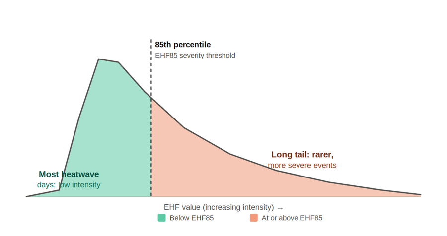
Fig G-1: Illustrative distribution of 85^th percentile of EHF values.

Annex H — Setting up the automatic warning flag

This annex covers only the logic of the warning flag — what triggers it and why. A separate article in this series is planned specifically on how AI-based forecasting tools can help automate this step once a threshold is in place; that article will address the practical build, not the underlying decision rule set out here.

Once a threshold is established (nodes I–K), the operational task is to integrate the EHF calculation into a daily, near-real-time workflow. In practice this means running the calculation on incoming weather observations and on short-range forecasts and setting an automatic flag when the three-day mean temperature is forecast to exceed the 95th percentile threshold (EHI_sig > 0), which flags “hotter than the seasonal norm”, in combination with short-term acclimatisation stress (EHI_accl > 0), which flags “hotter than the recent month”. Why both? Requiring both is what distinguishes a genuine heatwave signal from either a normal seasonal peak or a short hot spell after a mild patch.

Because EHF is an anomaly-based index, it can be calculated on forecast data as well as observed data — this is what gives can give a two- to five-day warning window rather than a purely retrospective identification of events, and is the operational advantage that justifies the derivation effort described in nodes A–L.

Annex I — Multi-sector validation and engagement

Node L asks you to validate the threshold against independent evidence and to share it. Health data is the most commonly used source, but it is not the only one, and other sectors often hold operational thresholds of their own that can corroborate — or usefully challenge — the derived EHF threshold:

• Health: where mortality or hospital admission data exists, even for a subset of years, check whether periods when EHF exceeded the severe threshold correspond to elevated all-cause mortality or heat-related admissions. This does not require a formal epidemiological study — a simple comparison is enough to give operational confidence.
• Power and energy infrastructure: ask plant operations engineers about the loss of cooling efficiency in evaporative cooling systems at high heat and humidity levels — many utilities already track this internally for maintenance planning, and it is a directly comparable, independently derived heat-humidity threshold.
• Agriculture: check with national agricultural extension or research services for known crop-specific thresholds, particularly night-time temperature thresholds during flowering (rice, wheat, maize and other staples are all vulnerable at this stage) and general livestock heat-stress thresholds.
• Transport and other infrastructure: where available, records of heat-related speed restrictions, rail buckling, or road surface failures can provide a further, independent cross-check on the severity threshold.

None of this is required before a threshold can be used operationally — node L’s documentation and health-data validation is the minimum. But where these sector contacts already exist, drawing on them costs little and materially strengthens the case that the threshold reflects something real, not just a statistical artefact of the derivation method.

References

Cannon, A.J. (2018) ‘Multivariate quantile mapping bias correction: an N-dimensional probability density function transform for climate model simulations of multiple variables’, Climate Dynamics, 50(1–2), pp. 31–49.

Debone, D., do Rosário, N.M.É. and Miraglia, S.G.E.K. (2025) ‘The Cost of Heat: Health and Economic Burdens in Three Brazilian Cities’, Atmosphere, 16(7), 755. Available at: https://doi.org/10.3390/atmos16070755 (Accessed: July 2026).

Lawrence, M.G. (2005) ‘The relationship between relative humidity and the dewpoint temperature in moist air: a simple conversion and applications’, Bulletin of the American Meteorological Society, 86(2), pp. 225–233.

Nairn, J.R. and Fawcett, R.J.B. (2015) ‘The Excess Heat Factor: A Metric for Heatwave Intensity and Its Use in Classifying Heatwave Severity’, International Journal of Environmental Research and Public Health, 12(1), pp. 227–253.

Nairn, J., Ostendorf, B. and Bi, P. (2018) ‘Performance of Excess Heat Factor Severity as a Global Heatwave Health Impact Index’, International Journal of Environmental Research and Public Health, 15(11), 2494.

Nairn, J., Moise, A. and Ostendorf, B. (2022) ‘The impact of humidity on Australia’s operational heatwave services’, Climate Services, 27, 100315. Available at: https://doi.org/10.1016/j.cliser.2022.100315 (Accessed: July 2026)

Oliveira, A., Lopes, A. and Soares, A. (2022) ‘Excess Heat Factor climatology, trends, and exposure across European Functional Urban Areas’, Weather and Climate Extremes, 36, 100455. Available at: https://doi.org/10.1016/j.wace.2022.100455 (Accessed: July 2026).

Thomas, N.P., Marquardt Collow, A.B., Bosilovich, M.G. and Dezfuli, A. (2023) ‘Effect of Baseline Period on Quantification of Climate Extremes Over the United States’, Geophysical Research Letters, 50, e2023GL105204.

World Health Organization and World Meteorological Organization (2025) Climate Change and Workplace Heat Stress. Geneva: WHO/WMO. Published 22 August 2025.

World Health Organization Regional Office for Europe (2026) Heat–Health Action Plans: Guidance, 2nd edn. Copenhagen: WHO Europe. Launched Berlin, 11 June 2026. ISBN 978-92-890-6293-0.

World Meteorological Organization (WMO) (2017) Guidelines on the Calculation of Climate Normals, WMO-No. 1203. Geneva: WMO.

World Meteorological Organization and World Health Organization (2015) Heatwaves and Health: Guidance on Warning-System Development, WMO-No. 1142. Geneva: WMO/WHO.

Zhang, X., Hegerl, G., Zwiers, F.W. and Kenyon, J. (2005) ‘Avoiding inhomogeneity in percentile-based indices of temperature extremes’, Journal of Climate, 18(8), pp. 1641–1651. Available at: https://doi.org/10.1175/JCLI3366.1 (Accessed: July 2026)

Zuo, Z., Li, Z., Ng, E.Y.Y., Ren, C. and Fung, J.C.H. (2026) ‘Humidity-enhanced Excess Heat Factor (EHF) analysis for heatwaves in the Pearl River Delta with CMIP6-WRF dynamical downscaling’, Weather and Climate Extremes, 100907. Available at: https://doi.org/10.1016/j.wace.2026.100907.